Characterizing the enzymatic clean up and ligation sequence bias
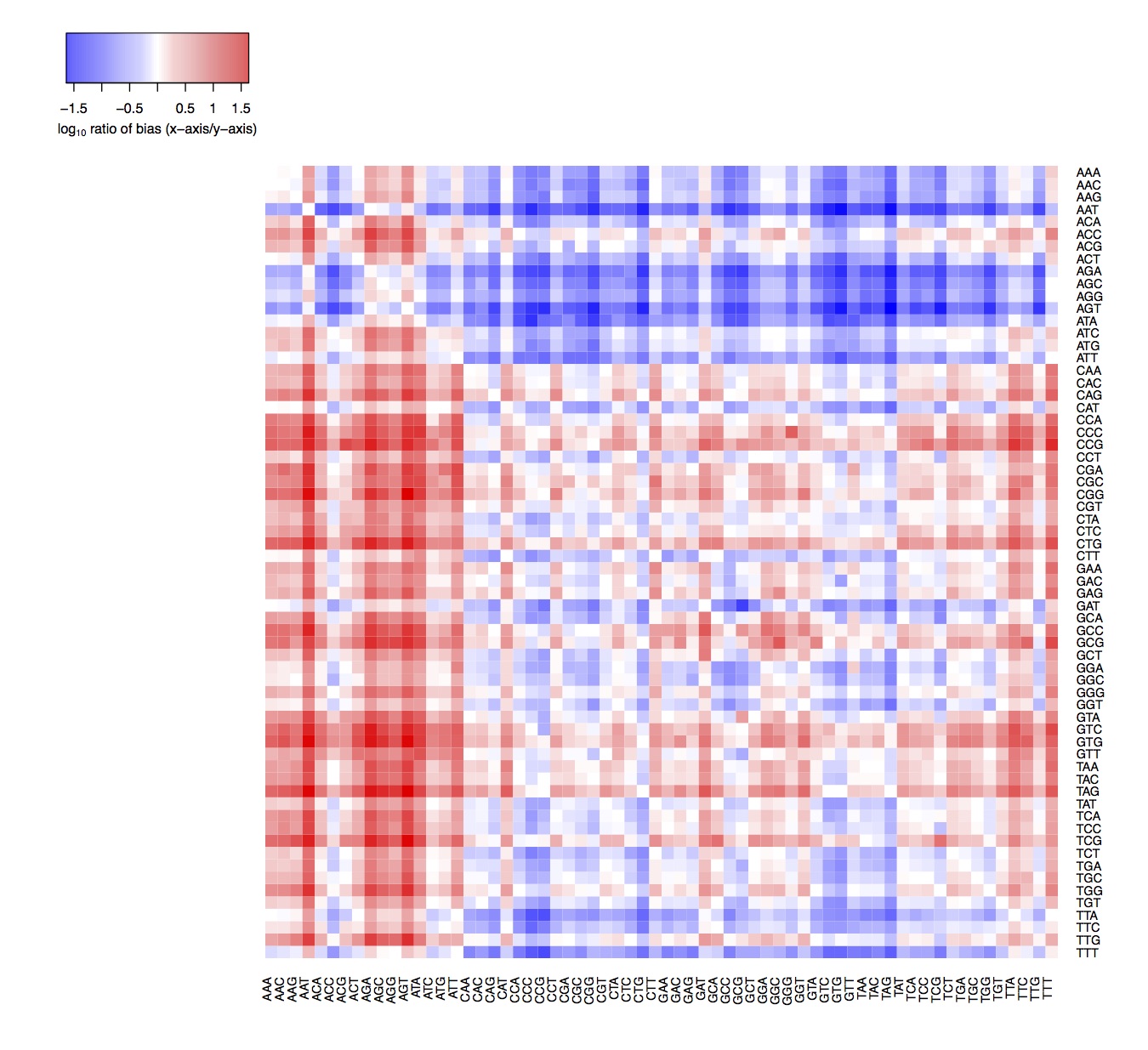
We had previously assumed that the three bases upstream and downstream of a DNase-nick site are equally likely to have adapters ligated and to be sequenced (Figure 2). However, we find that this is not the case and there is a bias in which 3-mer is ultimately detected by sequencing. Note that there is no inbalance for reverse palindromic 6-mers, for example: GCATGC
Plotting post-nicking enzymatic sequence biases
For each DNA nick we tally the number of times a plus strand and minus strand read detects the nick event. For simplicity, we assume that the mappability of plus and minus strand-aligned reads are the same. The analysis below is exclusively for the plus strand analysis, but a minus or combined strand analysis gives the same results.
source('https://raw.githubusercontent.com/guertinlab/seqOutBias/master/docs/R/seqOutBias_functions.R')
counts.table = read.table('~/DNase_ENCODE/hg38_36.6.3.3.IMR90_Naked_DNase.txt')
ligation = cbind(counts.table, substring(counts.table[,2],1,3))
ligation[,8] = apply(ligation, 1, function(row) revcomp(row[7]))
ligation[,9] = substring(counts.table[,2],4,6)
colnames(ligation) = c(colnames(counts.table), 'V7', 'rcKmerUp','KmerDown')
mat = data.frame(matrix(nrow=64, ncol= 64))
count = 0
for (mer in unique(ligation$KmerDown)) {
count = count + 1
temp = ligation[ligation$KmerDown == mer,] rto = temp[,6]/temp[,5]
mat[,count] = rto
}
colnames(mat) = unique(ligation$KmerDown)
mat = do.call(data.frame,lapply(mat, function(x) replace(x, is.infinite(x),NA)))
rownames(mat) = unique(temp[,8])
mat = mat[order(rownames(mat)) , order(colnames(mat))]
mat = as.matrix(mat)
pdf('lig_bias_matrix.pdf', width=10.4, height=9.5)
heatmap.2(log(mat, base=10), col=colorpanel(30, "blue", "white","red"),
symbreaks=T,scale="none",na.rm=TRUE,dendrogram = 'none', symm =TRUE,
density.info=c("none"), key.xlab = expression('log'[10]*' ratio of bias (x-axis/y-axis)'),
key.title= '',trace=c("none"),Rowv = FALSE, lhei=c(0.75,4), lwid = c(1.2, 4))
dev.off()
pdf('lig_bias_matrix_row.pdf', width=10.4, height=9.5)
heatmap.2(log(mat, base=10), col=colorpanel(30, "blue", "white","red"),
symbreaks=T,scale="none",na.rm=TRUE,dendrogram = 'row', symm =TRUE,
density.info=c("none"), key.xlab = expression('log'[10]*' ratio of bias (x-axis/y-axis)'),
key.title= '',trace=c("none"), Rowv = TRUE, lhei=c(0.75,4), lwid = c(1.2, 4))
dev.off()
n.diag = mat
diag(n.diag) = NA
df = data.frame(x=c(n.diag, diag(mat)), group=factor(c(rep("non-Palindromic", length(n.diag)),
rep("Palindromic", length(diag(mat))))))
pdf('lig_bias_bwplot.pdf', width=3, height=4)
trellis.par.set(box.umbrella = list(lty = 1, col="black", lwd=2),
box.rectangle = list(col = 'black', lwd=1.6),plot.symbol = list(col='black', lwd=1.6, pch ='.'))
bwplot(log(x, base = 2) ~ group, df,
scales=list(x=list(relation = "free", rot = 45)),
ylab = expression('log'[2]*' ratio of detection bias'),
pch = '|',
col= 'black' )
dev.off()
pdf('avg_ligation_bias.pdf', width=12, height=4)
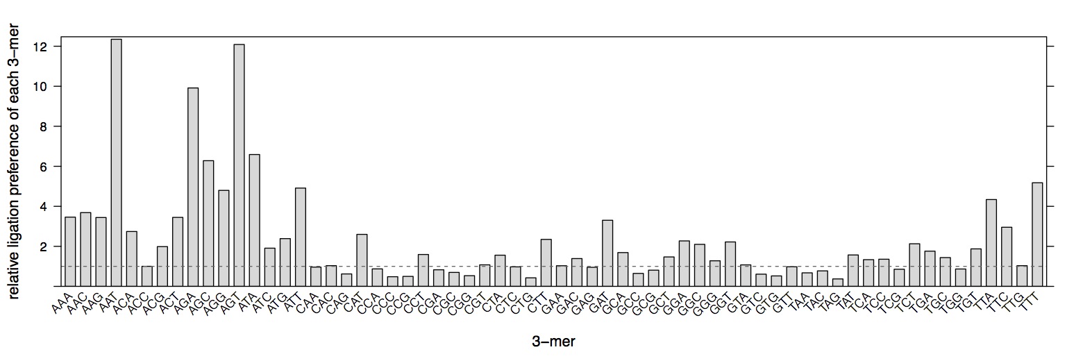
print(barchart((colMeans(mat, na.rm =TRUE)~colnames(mat)),
col='grey85',
ylim = c(0, max(colMeans(mat, na.rm =TRUE))+ 0.01 * max(colMeans(mat, na.rm =TRUE))),
ylab=paste('relative ligation preference of each 3-mer', sep = ' '),
xlab = '3-mer',
origin = 0,
scales=list(x=list(rot=45)),
panel=function(...) {
panel.barchart(...)
panel.abline(h=1, lty= 2, col = 'grey40')
}
))
dev.off()
#for (mer in unique(ligation$KmerDown)) {
for (mer in c('AAA', 'ATA', 'ATC', 'GAT','GAC')) {
plot.barchart.lig(ligation[ligation$KmerDown == mer,],
filename=paste('ligation_bias_',mer,'.pdf', sep = ''), w = 12, h = 4)
}
ligation$ratio = ligation[,6]/ligation[,5]
x.ligation = ligation[with(ligation, order(ratio)), ]
pswm.func(head(x.ligation[,2], 205), out = 'low_205.txt', positions = 6) pswm.func(tail(x.ligation[,2], 205), out = 'high_205.txt', positions = 6)

Testing whether 3’ and 5’ ssDNA overhangs contribute to enzymatic sequence bias
Preparing digested DNA for Illumina high throughput sequencing requires several enzymatic treatments. T4 DNA Polymerase treatment blunts ends by 3’ overhang removal and 3’ recessed (5’ overhang) end fill-in. T4 Polynucleotide kinase phosphorylates the 5’ end and Klenow Fragment (3’ to 5’ exo-) adds an A 5’ overhang. We hypothesized that the ligation preference for each 3-mer relative to all other 3-mers is dictated by the overhanging sequence. Although 4 nick events are necessary to sequence a DNA molecule, we only detect one nick on each end of the molecule and it is impossible to determine the precise location of the other nicks. By assuming that two enzymes with similar nick specificity (Figure 18) will have comparable distribution of sequence overhangs, we can test the hypothesis that the overhang sequences are contribute to post-nicking enzymatic treatment biases. Therefore, we compared this post-nicking bias using DNase-seq data from two different labs and two different organisms (Figure 19 and Figure 20). We also compared the biases of Cyanase and Benzonase (Figure 19 and Figure 20), which have similar sequence preferences (Figure 18), although Cyanase and Benzonase are distinct enzymes. Benzonase is an endonuclease cloned from Serratia marcescens. Cyanase is within the same evolutionary family of alpha/alpha/beta folded nucleases as Benzonase, but Cyanase is cloned from a non-Serratia species. Cyanase is active as a monomer and Benzonase is active as a dimer.
 seqOutBias table mm10_35.6.3.3.tbl mm10_liver_Cyanase.bam > mm10_35.6.3.3.liver_Cyanase.txt
 seqOutBias table mm10_35.6.3.3.tbl mm10_liver_Benzonase.bam > mm10_35.6.3.3.liver_Benzonase.txt
 seqOutBias table mm10_35.6.3.3.tbl mm10_liver_DNase.bam > mm10_35.6.3.3.liver_DNase.txt
setwd('~/TACh_Grontved')

counts.table.cyanase = read.table('mm10_35.6.3.3.liver_Cyanase.txt') counts.table.benzonase = read.table('mm10_35.6.3.3.liver_Benzonase.txt') counts.table.mm10.dnase = read.table('mm10_35.6.3.3.liver_DNase.txt')

totals.cyanase = colSums(counts.table.cyanase[,3:6])
scale.table.cyanase = data.frame(counts.table.cyanase[,1:2], t(apply(counts.table.cyanase[,3:6], 1,
    function(row) c((row[1]/totals[1]) / (row[3] / totals[3]), (row[2] / totals[2]) / (row[4] / totals[4])))))

totals.benzonase = colSums(counts.table.benzonase[,3:6])
scale.table.benzonase = data.frame(counts.table.benzonase[,1:2], t(apply(counts.table.benzonase[,3:6], 1,
    function(row) c((row[1]/totals[1]) / (row[3] / totals[3]), (row[2] / totals[2]) / (row[4] / totals[4])))))

totals.dnase = colSums(counts.table.mm10.dnase[,3:6])
scale.table.mm10.dnase = data.frame(counts.table.mm10.dnase[,1:2], t(apply(counts.table.mm10.dnase[,3:6], 1,
    function(row) c((row[1]/totals[1]) / (row[3] / totals[3]), (row[2] / totals[2]) / (row[4] / totals[4])))))

pdf('Cyanase_Benzonase_scale.pdf', width=4.5, height=4.5)
xyplot(log(scale.table.cyanase[,3], base = 10) ~ log(scale.table.benzonase[,3], base = 10),
        ylab = expression('log'[10]*'(Cyanase Scale Factor)'), xlab = expression('log'[10]*'(Benzonase Scale Factor)'),
        panel = function(x, y) {
            panel.xyplot(x, y,pch= 16, cex =0.5, col = 'black')
            panel.text(0.2*max(x), 0.95*min(y), label=paste('R = ', round(cor(x, y),2), sep =''))
        })
dev.off()

scale.table.dnase = do.call(data.frame,lapply(scale.table, function(x) replace(x, is.infinite(x),NA)))

pdf('DNase_Benzonase_scale.pdf', width=4.5, height=4.5)
xyplot(log(scale.table.dnase[,3], base = 10) ~ log(scale.table.benzonase[,3], base = 10),
    ylab = expression('log'[10]*'(MCF7 DNase Scale Factor)'), xlab = expression('log'[10]*'(Benzonase Scale Factor)'),
    panel = function(x, y) {
        panel.xyplot(x, y,pch= 16, cex =0.5, col = 'black')
        panel.text(-1.7, -1, label=paste('R = ', round(cor(x, y, use = 'complete.obs'),2), sep =''))
    })
dev.off()

pdf('DNase_DNase_mm10_scale.pdf', width=4.5, height=4.5)
xyplot(log(scale.table.dnase[,3], base = 10) ~ log(scale.table.mm10.dnase[,3], base = 10),
    ylab = expression('log'[10]*'(MCF7 DNase Scale Factor)'),
    xlab = expression('log'[10]*'(mouse liver DNase Scale Factor)'), panel = function(x, y) {
        panel.xyplot(x, y,pch= 16, cex =0.5, col = 'black')
        panel.text(0.4, -1, label=paste('R = ', round(cor(x, y, use = 'complete.obs'),2), sep =''))
})
dev.off()

cyanase.mat = matrix.func(counts.table.cyanase)
benzonase.mat = matrix.func(counts.table.benzonase)
dnase.mcf7.mat = matrix.func(counts.table)
dnase.mm10.mat = matrix.func(counts.table.mm10.dnase)

pdf('lig_bias_matrix_benzonase.pdf', width=10.4, height=9.5)
    heatmap.2(log(benzonase.mat, base=10), col=colorpanel(100, "blue", "white","red"),
    symbreaks=T,scale="none",na.rm=TRUE,dendrogram = 'none', symm =TRUE,
    density.info=c("none"), key.xlab = expression('log'[10]*' ratio of bias (x-axis/y-axis)'),
    key.title= '',trace=c("none"),Rowv =FALSE, lhei=c(0.75,4), lwid = c(1.2, 4))
dev.off()

pdf('lig_bias_matrix_cyanase.pdf', width=10.4, height=9.5)
heatmap.2(log(cyanase.mat, base=10), col=colorpanel(100, "blue", "white","red"),
    symbreaks=T,scale="none",na.rm=TRUE,dendrogram = 'none', symm =TRUE,
    density.info=c("none"), key.xlab = expression('log'[10]*' ratio of bias (x-axis/y-axis)'),
    key.title= '',trace=c("none"),Rowv =FALSE, lhei=c(0.75,4), lwid = c(1.2, 4))
dev.off()

pdf('lig_bias_matrix_dnase_mcf7.pdf', width=10.4, height=9.5)
heatmap.2(log(dnase.mcf7.mat, base=10), col=colorpanel(100, "blue", "white","red"),
    symbreaks=T,scale="none",na.rm=TRUE,dendrogram = 'none', symm =TRUE,
    density.info=c("none"), key.xlab = expression('log'[10]*' ratio of bias (x-axis/y-axis)'),
    key.title= '',trace=c("none"),Rowv =FALSE, lhei=c(0.75,4), lwid = c(1.2, 4))
dev.off()

pdf('lig_bias_matrix_dnase_mm_liver.pdf', width=10.4, height=9.5)
heatmap.2(log(dnase.mm10.mat, base=10), col=colorpanel(100, "blue", "white","red"),
    symbreaks=T,scale="none",na.rm=TRUE,dendrogram = 'none', symm =TRUE,
    density.info=c("none"), key.xlab = expression('log'[10]*' ratio of bias (x-axis/y-axis)'),
    key.title= '',trace=c("none"),Rowv =FALSE, lhei=c(0.75,4), lwid = c(1.2, 4))
dev.off()

pdf('DNase_DNase_comparison_post_nick.pdf', width=4.5, height=4.5)
xyplot(as.numeric(unlist(log(dnase.mm10.mat, base = 10))) ~ as.numeric(unlist(log(dnase.mcf7.mat, base = 10))),
    ylab = expression('log'[10]*'(mouse liver DNase ratio bias)'),
    xlab = expression('log'[10]*'(MCF7 DNase ratio bias)'),
    panel = function(x, y) {
        panel.xyplot(x, y,pch= 16, cex =0.5, col = 'black')
        panel.text(1, -1.5, label=paste('R = ', round(cor(x, y, use = 'complete.obs'),2), sep =''))
    })
dev.off()

pdf('Cyanase_Benzoase_comparison_post_nick.pdf', width=4.5, height=4.5)
xyplot(as.numeric(unlist(log(cyanase.mat, base = 10))) ~ as.numeric(unlist(log(benzonase.mat, base = 10))),
    ylab = expression('log'[10]*'(Cyanase ratio bias)'),
    xlab = expression('log'[10]*'(Benzonase ratio bias)'),
    panel = function(x, y) {
        panel.xyplot(x, y,pch= 16, cex =0.5, col = 'black')
        panel.text(1, -1.5, label=paste('R = ', round(cor(x, y, use = 'complete.obs'),2), sep =''))
    })
dev.off()

pdf('DNase_Benzoase_comparison_post_nick.pdf', width=4.5, height=4.5)
xyplot(as.numeric(unlist(log(dnase.mcf7.mat, base = 10))) ~ as.numeric(unlist(log(benzonase.mat, base = 10))),
    ylab = expression('log'[10]*'(MCF7 DNase ratio bias)'),
    xlab = expression('log'[10]*'(Benzonase ratio bias)'),
    panel = function(x, y) {
        panel.xyplot(x, y,pch= 16, cex =0.5, col = 'black')
        panel.text(1, -1.5, label=paste('R = ', round(cor(x, y, use = 'complete.obs'),2), sep =''))
    })
dev.off()


In conclusion, we show that seqOutBias successfully corrects sequence bias associated with many molecular genomics techniques and our analysis indicate that the enzymes that are common to many library prepartion protocols exhibit previously uncharacterized biases.