seqOutBias

Vignette

by Guertin Lab

⇦ Contents ⇨

`seqOutBias` to generate scaled bigWig files

The software seqOutBias will scale aligned bam read counts by the ratio of genome-wide observed read counts to the sequence based counts for each k-mer. The k-mer counts take into account the mappability at a given read length. The seqOutBias program allows for flexibility in specifying k-mer size, strand-specific offsets, and spaced k-mers.

Using `seqOutBias` to scale DNase-seq files by 6-mer nick preference

The specificity of DNase is strongly influenced by the three bases that flank each side of the DNase cut site (Figure 1) (He et al., 2014; Yardımcı et al., 2014).

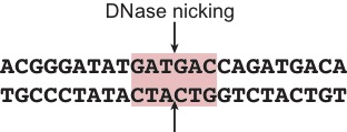
Figure 1: The six base pair window centered on the DNase nick dictates cleavage preference. (He *et al.*, 2014)

seqOutBias will calculate the genome-wide occurences of each specified k-mer centered on the DNase nick site accounting for the mappability of the specified read length (note the default is –read-size=36). For each case below the offsets are half the value of the kmer-size parameter, which is the sequence length (k-mer) that surronds the nick-site and influences specificity, therefore the program will calculate the frequency of k-mers centered on the nick-site. Experimentally, we assume that we are equally likely to sequence either end of a DNase nick site, so the –shift-counts parameter is used to shift the Crick strand alignments in line with the Watson strand alignments (Figure 2). DNase nicks can be offset or in line, as shown. Note that generating the mappability files for a given genome and read length is time-consuming, but once these files are made, seqOutBias will recognize the existence of these files and avoid timely recomputing and regeneration of these files.

bam=UW_MCF7_both.bam
`seqOutBias` hg38.fa $bam --no-scale --bw=MCF7_0-mer.bigWig --shift-counts --skip-bed
`seqOutBias` hg38.fa $bam --kmer-size=6 --bw=MCF7_6-mer.bigWig --plus-offset=3 --minus-offset=3 --shift-counts --skip-bed
`seqOutBias` hg38.fa $bam --kmer-size=10 --bw=MCF7_10-mer.bigWig --plus-offset=5 --minus-offset=5 --shift-counts --skip-bed
bam=IMR90_Naked_DNase.bam
`seqOutBias` hg38.fa $bam --no-scale --bw=Naked_0-mer.bigWig --shift-counts --skip-bed
`seqOutBias` hg38.fa $bam --kmer-size=6 --bw=Naked_6-mer.bigWig --plus-offset=3 --minus-offset=3 --shift-counts --skip-bed
`seqOutBias` hg38.fa $bam --kmer-size=10 --bw=Naked_10-mer.bigWig --plus-offset=5 --minus-offset=5 --shift-counts --skip-bed

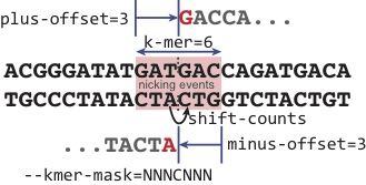
Figure 2: DNase nicking occurs as marked between the two centered base pairs. DNase’s specificity is conferred by the hexamer sequence centered (red block) on the nick sites (dotted vertical lines); this parameter is referred to as the `k-mer`. For the purposes of this illustration, the two nicks that result in liberation of the DNA ends are in line. We explore the scenarios where the nicks are offset and result in overhangs in Section 8. The `plus-offset` and `minus-offset` specify the nick site relative to the first position and last position of the `k-mer`. During the library preparation, we assume that the plus and minus strand are equally likely to be sequenced (either red nucleotide will be the first base sequenced). This assumption, however, is not true and the DNA end-repair and ligation have inherent biases. As opposed to specifying the immediate upstream base for the minus strand, we arbitrarily shift the base position by +1 to match the position of the immediate upstream base from the plus aligned read; note that the actual shift amounts will differ depending on the relative positions dictated by the plus/minus-offset values.

Visualizing the single-nucleotide cut files in UCSC

Convert the bigWig files to bedGraph and add a header to the files for loading into the UCSC genome browser. First use the UCSC tool bigWigToBedGrap to convert the bigWig files to bedGraph files, then add a header to the files, and compress.

for wig in *bigWig
do
    name=$(echo $wig | awk -F".bigWig" '{print $1}')
    echo $name
    touch temp.txt
    echo "track type=bedGraph name=$name" >> temp.txt
    bigWigToBedGraph $wig $name.bdg
    cat temp.txt $name.bdg > $name.bedGraph
    rm temp.txt
    rm $name.bdg
    gzip $name.bedGraph
done
mkdir Naked
mkdir MCF7
mv Naked*bigWig Naked
mv MCF7*bigWig MCF7

Use the UCSC browser to visualize the normalized and unnormalized files (Karolchik et al., 2014). Click Genomes in the upper left corner (Figure 3). Make sure you have the correct assembly, we are using hg38. Next click add custom tracks (Figure 4). Use the GUI to navigate to the *.bedGraph.gz file-containing directory and upload each file individually. You will want to register and save sessions and you will only need to upload the data once.

Figure 4: Below the browser, click the **add custom tracks** icon.

Figure 5: Note that each bar is scaled inversely with DNase sequence preference.

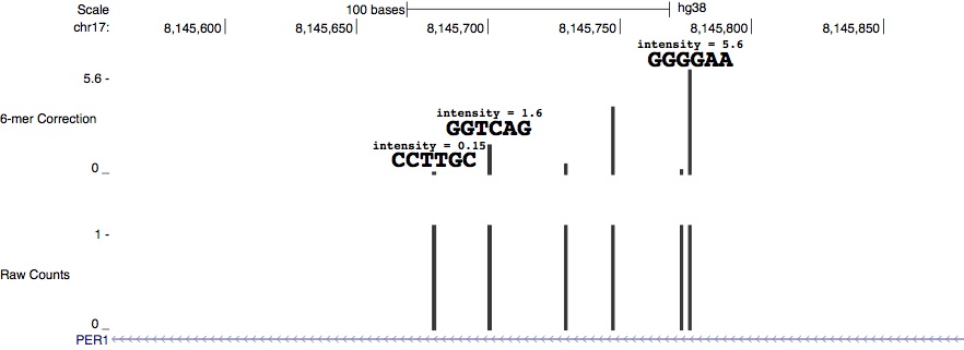
Generating and analyzing k-mer count tables

Next you can use seqOutBias table to generate a table that contains the k-mer index, k-mer string, plus strand count, minus strand count, observed plus strand reads, and observed minus strand reads.

seqOutBias table hg38_36.6.3.3.tbl IMR90_Naked_DNase.bam > hg38_36.6.3.3.IMR90_Naked_DNase.txt

Compare the frequency of the 4096 hexamers in the genome with the observed cut frequency of DNase using R.

setwd('~/DNase_ENCODE')

counts.table = read.table('hg38_36.6.3.3.IMR90_Naked_DNase.txt')
totals = colSums(counts.table[,3:6])
scale.table = data.frame(counts.table[,1:2], t(apply(counts.table[,3:6], 1,
    function(row) c((row[1]/totals[1]) / (row[3] / totals[3]), (row[2] / totals[2]) / (row[4] / totals[4])))))

scale.table[scale.table[,2] == 'CCTTGC',]
scale.table[scale.table[,2] == 'GGTCAG',]
scale.table[scale.table[,2] == 'GGGGAA',]

Retrieving ChIP-seq binding and sequence motif data

To look at composite footprints that result from transcription factor binding to DNA in the context of chromatin, we need to first find all the regions bound by the factor. We get these from processed ENCODE data; we could merge or intersect the replicate files using software like bedtools (Quinlan and Hall, 2010), but for the purposes of this vignette we will keep it simple and look at the first replicate broadPeak file for three factors. We need to convert these files from hg19 to hg38 coordinates using UCSC liftOver and retrieve the sequence associated with each genome coordinate using fastaFromBed from bedtools (Quinlan and Hall, 2010). Note that we use MAST (Bailey et al., 2009) to identify TF binding sites within ChIP-seq peaks to infer the site of TF binding precisely using traditional DNase-seq data. However, since the naked DNA DNase-seq is lower coverage and the DNA was stripped of proteins, we use FIMO (Grant et al., 2011) to identify all potential TF binding sites in the genome for our composite profiles.

url=http://hgdownload.cse.ucsc.edu/goldenPath/hg19/encodeDCC/wgEncodeHaibTfbs/ wget ${url}wgEncodeHaibTfbsMcf7Elf1V0422111PkRep1.broadPeak.gz
wget ${url}wgEncodeHaibTfbsMcf7Gata3V0422111PkRep1.broadPeak.gz
wget ${url}wgEncodeHaibTfbsMcf7MaxV0422111PkRep1.broadPeak.gz
wget ${url}wgEncodeHaibTfbsMcf7CtcfcV0422111PkRep1.broadPeak.gz
wget http://hgdownload.cse.ucsc.edu/goldenPath/hg19/liftOver/hg19ToHg38.over.chain.gz gunzip hg19ToHg38.over.chain.gz

for peak in *Rep1.broadPeak.gz do
    name=$(echo $peak | awk -F"wgEncodeHaibTfbsMcf7" '{print $NF}' | awk -F"V0422111PkRep1.broadPeak.gz" '{print $1}') unz=$(echo $peak | awk -F".gz" '{print $1}')
    echo $name
    gunzip $peak
    echo $unz
    liftOver $unz hg19ToHg38.over.chain $name.hg38.broadPeak $name.hg38.unmapped.txt -bedPlus=6 fastaFromBed -fi hg38.fa -bed $name.hg38.broadPeak -fo $name.hg38.fasta
    gzip *broadPeak
done
mv Ctcfc.hg38.fasta CTCF.hg38.fasta

We are interested in those factor binding events that are direct and we will use the presence of a strong consensus binding motif as an indicator of direct binding. There are many potential sources for position specific weight matrices, but we will use MEME (Bailey et al., 2006).

wget http://meme-suite.org/meme-software/Databases/motifs/motif_databases.12.12.tgz
tar -xvf motif_databases.12.12.tgz
head -9 motif_databases/JASPAR/JASPAR_CORE_2016_vertebrates.meme > header_meme_temp.txt
grep -i -A 14 'MOTIF MA0058.3 MAX' motif_databases/JASPAR/JASPAR_CORE_2016.meme > max_temp.txt
grep -i -A 16 'MOTIF MA0473.2 ELF1' motif_databases/JASPAR/JASPAR_CORE_2016.meme > elf1_temp.txt
grep -i -A 12 'MOTIF MA0037.2 GATA3' motif_databases/JASPAR/JASPAR_CORE_2016.meme > gata3_temp.txt
grep -i -A 23 'MOTIF MA0139.1 CTCF' motif_databases/JASPAR/JASPAR_CORE_2016.meme > ctcf_temp.txt
cat header_meme_temp.txt ctcf_temp.txt > CTCF_minimal_meme.txt
cat header_meme_temp.txt max_temp.txt > Max_minimal_meme.txt
cat header_meme_temp.txt elf1_temp.txt > Elf1_minimal_meme.txt
cat header_meme_temp.txt gata3_temp.txt > Gata3_minimal_meme.txt
rm *temp.txt

for meme in *.hg38.fasta
do
    name=$(echo $meme | awk -F".hg38.fasta" '{print $1}')
    echo $name
    mast ${name}_minimal_meme.txt $meme -hit_list -mt 0.0005 > ${name}_mast.txt
    fimo --thresh 0.0001 --text ${name}_minimal_meme.txt hg38.fa > ${name}_fimo.txt
    ceqlogo -i1 ${name}_minimal_meme.txt -o ${name}_logo.eps -N -Y
done

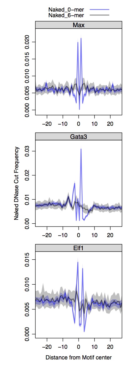
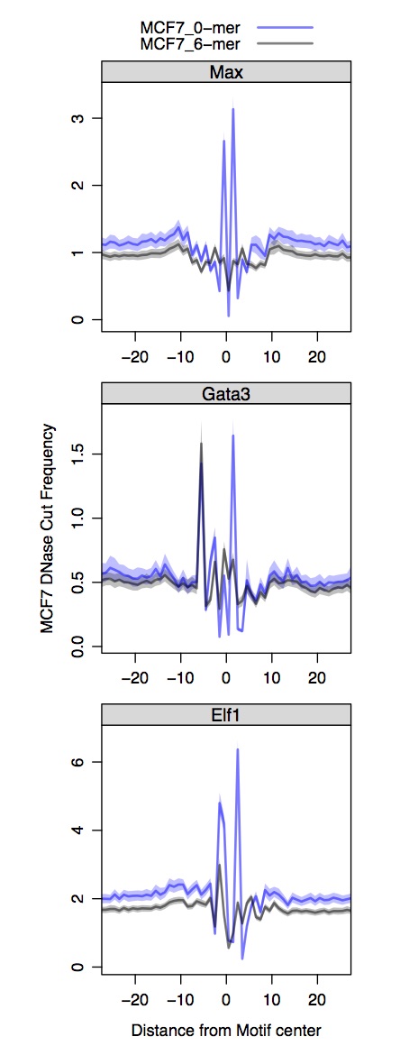
Use `R` to plot composite DNase profiles at TF binding sites

First you need to install the bigWig library from André Martins. The lattice and latticeExtra libraries can be installed from the CRAN repository. Recall we process the Naked DNA DNase-seq and conventional DNase-seq separately and the input motifs are distinct for each.

source('https://raw.githubusercontent.com/guertinlab/seqOutBias/master/docs/R/seqOutBias_functions.R')

#note that the full path is needed to the directory containing the bigWigs
all.composites.dnase.naked = cycle.fimo.new.not.hotspots(path.dir.fimo = '~/DNase_ENCODE/', path.dir.bigWig = '/Users/guertinlab/DNase_ENCODE/Naked/', window = 30, exp = 'Naked_DNase')
all.composites.dnase.mcf7 = cycle.fimo.new.not.hotspots(path.dir.mast = '~/DNase_ENCODE/', path.dir.bigWig = '/Users/guertinlab/DNase_ENCODE/MCF7/', window = 30, exp = 'MCF7_DNase')

composites.func.panels.naked.chromatin(all.composites.dnase.mcf7[(all.composites.dnase.mcf7$cond == 'MCF7_0-mer' | all.composites.dnase.mcf7$cond == 'MCF7_6-mer') & (all.composites.dnase.mcf7$grp != 'CTCF') ,],
fact = 'MCF7 DNase', summit = 'Motif', num = 24, col.lines = c(rgb(0,0,1,1/2), rgb(0,0,0,1/2)),
fill.poly = c(rgb(0,0,1,1/4), rgb(0,0,0,1/4)))

composites.func.panels.naked.chromatin(all.composites.dnase.naked[(all.composites.dnase.naked$cond == 'Naked_0-mer' | all.composites.dnase.naked$cond == 'Naked_6-mer') & (all.composites.dnase.naked$grp != 'CTCF'),],
fact= "Naked DNase", summit= "Motif",num = 24, col.lines = c(rgb(0,0,1,1/2), rgb(0,0,0,1/2)), fill.poly = c(rgb(0,0,1,1/4), rgb(0,0,0,1/4)))

save(all.composites.dnase.naked, all.composites.dnase.mcf7, '~/DNase_ENCODE/MCF7_composites.Rdata')

Figure 6: The DNase nick bias is abrogated in an deproteinized DNA (Naked) DNase experiment (Lazarovici *et al.*, 2013) as illustrated by these composite profiles of DNase cut-frequency for three distinct transcription factor motifs.

Figure 7: Upon correcting for DNase nick bias, we observe true signatures that may be a result of TF/protein interactions, which we do not observe with the Naked DNase composites. Note the sharp peak upstream of the GATA3 motif; this sharp signature peak is one base-pair downstream (position x = -5.5) of the broader and less intense signature peak observed in Figure 6 (position x = -6.5). Max exhibits a modest composite footprint, which is caused by protection from DNase activity mediated by TF/protein interaction.

seqOutBias to generate scaled bigWig files